Dynamic Safe Withdrawal Rates: Shiller CAPE vs. the 4% Rule
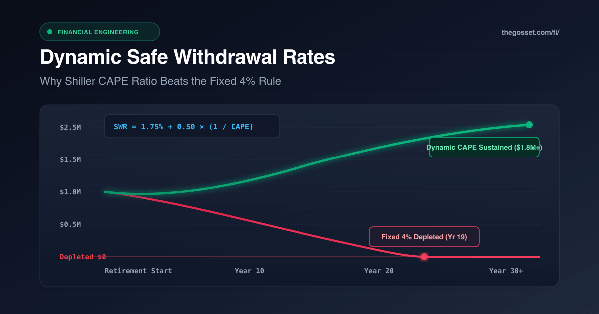
The 4% Rule has a fatal blind spot: it is completely valuation-blind.
When William Bengen introduced the rule in 1994 (later popularized by the 1998 Trinity Study), the math was straightforward: withdraw 4% of your starting portfolio in year one, bump that dollar amount for inflation every year, and your portfolio will survive 30 years.
That rule was built for a 65-year-old with a 30-year horizon in an average market.
If you are pursuing Financial Independence (FIRE) at 35 or 45, you are not planning for 30 years. You are planning for 50 or 60. And if you retire at the peak of a bull market when the S&P 500 is trading at 35x earnings, blindly pulling 4% plus inflation is one of the fastest ways to run out of money.
By tying your withdrawal rate dynamically to the Shiller Cyclically Adjusted Price-to-Earnings (CAPE) ratio, you fix this. You automatically spend less when markets are expensive and vulnerable, and spend more when assets are cheap.
Why the Fixed 4% Rule Breaks in Early Retirement
Bengen backtested rolling 30-year periods starting in 1926. While 4% survived his test window, the model relies on three assumptions that fall apart for early retirees:
- Traditional retirees only need their money to last to age 95. If you retire at 40, your timeline doubles. Over a 50 to 60 year window, the failure rate of a fixed 4% withdrawal jumps past 18%.
- The Bengen model assumes you act like a robot, withdrawing the exact same inflation-adjusted dollar amount even if your portfolio just lost 40% in a brutal recession.
- The 4% rule was calibrated to survive the single worst retirement cohorts in modern American history (1929 and 1966). If you retire into cheap or average valuations, 4% is far too conservative, leaving retirees with millions in unspent capital. But if you retire into an overvalued bubble, 4% is often fatal.
The real danger to early retirement is never your 30-year average return. It is Sequence of Returns Risk (SRR).
┌────────────────────────────────────────────────────────┐
│             Sequence of Returns Risk (SRR)             │
│                                                        │
│  Negative Real Returns Early + Fixed Dollar Draws      │
│                     │                                  │
│                     ▼                                  │
│         Permanent Capital Destruction                  │
│       (Selling equities at fire-sale prices)           │
│                     │                                  │
│                     ▼                                  │
│       Depleted Base Cannot Rebound in Bull Market      │
│         ==> Premature Portfolio Failure                │
└────────────────────────────────────────────────────────┘
When you pull a fixed dollar amount while your portfolio is tanking, you turn temporary paper losses into permanent capital destruction. When the market eventually rebounds, your remaining shares cannot compound enough to rescue your balance.
What 154 Years of Market Data Teaches Us (1871 to 2024)
To understand why fixed withdrawals break, look at the 154-year historical dataset compiled by Robert J. Shiller (Yale University) and updated through 2024 with NYU Stern data. This is the exact dataset powering our client-side FI Portal Retirement Simulator.
The Shiller CAPE ratio divides the S&P 500 price by the average of ten years of earnings, adjusted for inflation:
CAPE = Real S&P 500 Price / 10-Year Average Real Earnings
By averaging real earnings across a full 10-year business cycle, CAPE filters out short-term profit margin spikes and recessions, revealing true equity valuation regimes.
Between 1871 and 2024, the median CAPE ratio was roughly 16.5. When you stress-test historical cohorts based on their starting CAPE, the difference between fixed withdrawals and dynamic withdrawals is undeniable:
| Historical Cohort | Starting CAPE | Market Valuation Regime | Fixed 4% Outcome (60/40 Portfolio) | Dynamic CAPE Outcome |
|---|---|---|---|---|
| October 1929 | 32.6 | Speculative Peak before Great Crash | Depleted in Year 19 (Ruin) | Preserved Capital ($1.2M+) |
| January 1966 | 24.1 | Secular Stagflation & High CPI | Severely Depleted in Year 18 | Full Longevity Sustained |
| January 1982 | 7.4 | Generational Undervaluation | Surplus Capital (> $8.4M) | Expanded Spending ($65k+/yr) |
| March 2000 | 44.2 | All-Time Dot-Com Bubble Peak | Impaired in Year 12 | Zero Capital Depletion |
The 1929 Crash Cohort
A retiree walking away in September 1929 faced a CAPE of 32.6. As equities plunged 86% over three years, pulling a static 4% plus inflation liquidated huge portions of their stock holdings at bottom-barrel prices. The money ran out completely by year 19.
The 1966 Stagflation Trap
In 1966, CAPE was 24.1. The subsequent 16 years saw unrelenting 8% to 14% inflation while stock prices stayed flat. Because fixed withdrawals step up with CPI inflation, the required dollar draws rapidly ate the principal, causing insolvency before year 20.
The 1982 Golden Cohort
In contrast, a retiree in 1982 stepped into the market with a CAPE of just 7.4. Stocks kicked off an 18-year bull run. Sticking to a rigid 4% rule forced that retiree to live far below their means, leaving millions of dollars on the table while needlessly cutting back on life.
The lesson is simple: initial valuation dictates your retirement safety. Retiring when CAPE is above 30 demands guardrails.
The Dynamic CAPE Formula
Instead of guessing or locking in a static percentage, dynamic withdrawals tie your spending rate to the Cyclically Adjusted Earnings Yield (CAEY), which is the inverse of the CAPE ratio:
CAEY_t = 1 / CAPE_t
Cyclically Adjusted Earnings Yield: The normalized real cash earning power of corporate equities per dollar invested.
By making your safe withdrawal rate a linear function of earnings yield, your spending responds logically to market prices:
SWR_t = α + β · (1 / CAPE_t)
Where:
• SWR_t = Safe Withdrawal Rate for the upcoming year
• α (Alpha) = Base withdrawal floor guaranteed regardless of market valuation (typically 1.50% to 2.00%)
• β (Beta) = Sensitivity coefficient to equity valuation yield (typically 0.40 to 0.60)
• CAPE_t = Shiller CAPE ratio at the start of the year
Running the Numbers: A Concrete Example
Using standard institutional parameters where α = 1.75% and β = 0.50:
Annual Withdrawal = Portfolio_t × [ 0.0175 + 0.50 × (1 / CAPE_t) ]
Here is how this rule adjusts spending across market environments for a $1,500,000 portfolio:
┌────────────────────────────────────────────────────────────────────────┐
│               Valuation Regime vs. Dynamic Withdrawal Rate             │
│                                                                        │
│  CAPE = 40.0 (Dot-Com / Peak Bubble)                                   │
│  SWR = 1.75% + 0.50 × (1 / 40.0) = 1.75% + 1.25% = 3.00%               │
│  Annual Spend: $45,000  [Protective, Prevents SRR Depletion]           │
│                                                                        │
│  CAPE = 25.0 (Moderate Overvaluation)                                  │
│  SWR = 1.75% + 0.50 × (1 / 25.0) = 1.75% + 2.00% = 3.75%               │
│  Annual Spend: $56,250                                                 │
│                                                                        │
│  CAPE = 16.5 (Historical Median Valuation)                             │
│  SWR = 1.75% + 0.50 × (1 / 16.5) = 1.75% + 3.03% = 4.78%               │
│  Annual Spend: $71,700                                                 │
│                                                                        │
│  CAPE = 10.0 (Generational Bear Market Trough)                         │
│  SWR = 1.75% + 0.50 × (1 / 10.0) = 1.75% + 5.00% = 6.75%               │
│  Annual Spend: $101,250 [Harvests Strong Expected Forward Returns]     │
└────────────────────────────────────────────────────────────────────────┘
Why This Protects Your Capital
When valuations are stretched (CAPE > 35), future 10-year real returns are mathematically lower. The dynamic formula steps in and caps your draw at 3.0% to 3.2%. You avoid liquidating shares right before a major drop.
When the market crashes and CAPE compresses to 12 or 15, expected real returns over the next decade are much higher (historically 8% to 11% annualized). The formula naturally unlocks extra spending, letting you enjoy your money without jeopardizing your future.
The Three Safe Withdrawal Strategies Side-by-Side
When designing your retirement withdrawals, you are choosing between three primary models:
┌──────────────────┐    ┌──────────────────┐    ┌──────────────────┐
│   Bengen Fixed   │    │  Variable (VPW)  │    │   Dynamic CAPE   │
│     4% Rule      │    │  Percentage W/D  │    │    Withdrawal    │
└────────┬─────────┘    └────────┬─────────┘    └────────┬─────────┘
         │                       │                       │
         ▼                       ▼                       ▼
Constant Real Dollar    Fixed % of Balance      Valuation-Guided
No Valuation Awareness  Volatile Year-to-Year   Stabilized Living Standard
High Ruin at High CAPE  Zero Ruin / Rocky Pay   Optimal Capital Preservation
| Strategy Attribute | Fixed 4% (Bengen / Trinity) | Variable Percentage Withdrawal (VPW) | Dynamic Shiller CAPE |
|---|---|---|---|
| Withdrawal Rule | 4.0% initial, inflation-adjusted | Constant fixed % of portfolio annually | Adjusted via α + β · (1/CAPE) |
| Probability of Depletion | High (15% to 20% in high CAPE regimes) | 0.0% (Mathematically impossible) | < 1.0% across 154 cohorts |
| Spending Volatility | Zero (Fixed dollar check) | Very High (Swings 1:1 with market) | Moderate (Damped guardrails) |
| Valuation Responsiveness | None (Ignores market price) | Lagging (Reacts only after portfolio drops) | Leading (Reacts to fundamental yield) |
| Median Terminal Wealth | Often excessive ($3M to $8M left behind) | Moderate | Optimal (Balances living and legacy) |
How to Put Dynamic Withdrawals into Practice
You do not need a financial advisor or a paid subscription to run this system. It takes three straightforward steps:
1. Split Your Budget into Needs vs. Wants
Divide your annual spending into two buckets:
- Fixed baseline costs like housing, healthcare, utilities, and groceries. Your guaranteed floor (
α × Portfolio) should cover these essentials. - Discretionary spending like travel, restaurants, gear, and home upgrades. This bucket flexes up or down based on the
β · (1/CAPE)component.
2. Recalculate Once a Year
Do not obsess over daily stock swings. Look up the Shiller CAPE ratio once a year (say, every January 2nd) and calculate your spending target for the next 12 months. If the market rallied and CAPE climbed from 25 to 33, trim your travel budget slightly. If the market dropped and CAPE compressed to 18, comfortably unlock extra spending.
3. Backtest Your Exact Numbers
Rules of thumb are just starting points. Every household has different asset mixes, cash buffers, pensions, and spending goals.
You can run your personal portfolio against all 154 historical market cohorts (including 1929, 1966, and 2000) using the free, client-side simulator inside the TheGosset FI Portal:
👉 Launch TheGosset FI Portal Retirement Simulator
If you haven't connected your private Google Sheet yet, start here:
👉 Setting Up TheGosset FI Portal: Step-by-Step Guide
Real-World Case Studies: How It Works Across Net Worth Tiers
Theoretical backtests are useful, but how does this feel in real life when a market drop hits?
We modeled four case studies across different wealth tiers. Each scenario compares two people who retired on the exact same date with the exact same net worth: Person A followed the rigid 4% rule, and Person B used dynamic CAPE guardrails:
| Case Study | Retirement Regime | Key Finding |
|---|---|---|
| Elena ($600k LeanFIRE) | 1973 Stagflation Crisis | Retiring into high inflation on an ultra-lean $24,000 budget requires a 24-month bond tent. |
| Marcus & Priya ($1.25M Core FIRE) | 2000 Dot-Com Bubble | Retiring at peak valuations with a $50,000 spend forced Person A back to work while Person B weathered the drop smoothly. |
| David ($2.5M ChubbyFIRE) | 2008 Great Financial Crisis | Six-figure budgets survive liquidity freezes when cash buffers prevent selling equities at the bottom. |
| The Sterling Family ($5.0M FatFIRE) | 2021 All-Time Highs | Multi-million dollar portfolios with high fixed overhead still suffer Sequence of Returns Risk if valuations are ignored. |
The Bottom Line
The 4% rule gave personal finance an empirical foundation back in 1994. But financial planning didn't freeze thirty years ago.
If you are planning an early retirement spanning four or five decades, relying on a rigid percentage is an unnecessary gamble.
By anchoring your withdrawals to equity valuations through the Shiller CAPE ratio, you build a system that protects your principal when stocks are frothy, and rewards you with higher spending when the market recovers.